Determining plate fin heat sinks parameters

Heat sink

Often heat needs to be extracted from an embedded system to increase lifetime and performance. Heat extracting methods include active and passive heat sink cooling, thermoelectric cooling, water cooling, heat pipes and phase-change cooling. Every method has its advantages and disadvantages.

Passive cooling using plate fin sinks is a fail safe and quiet method that consumes no power and is easy to manufacture. This article describes how to use the physics and mathematics behind a plate fin sin sink to design a sufficient cooling device for an embedded system.

The discussion is based on an embedded system with a power consumption of 12 W. The system is mounted in an aluminum casing with a flat 245 mm times 290 mm surface, a suitable place to mount the heat sink. The heat sink is there to keep the system temperature within acceptable levels. An acceptable temperature level in this case is typically between 30 degrees and 50 degrees Celsius depending on hardware and component temperature restrictions.

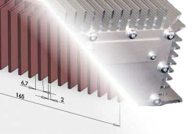
Extracting heat by natural convection

The temperature can only be kept within the limits by extracting heat through conduction, convection or radiation. Plate fin sinks extract heat by natural convection. Heat spreading is essentially area enlarging. The larger the area the more energy can be removed at the same temperature difference.

Unfortunately calculating the natural convection heat transfer for a specific plate fin heat sink is not that simple. A lot of constraints have influence on the heat flow, such as geometry, material properties, and the boundary and ambient conditions. The physics of such a model is described in detail further down in the text.

Web based simulation tool

Luckily there are easier ways to perform the calculations. The situation is often simplified in a model where isothermal boundary conditions are assumed to uniformly apply over the back surface of the base plate.The Microelectronic Heat Transfer Laboratory of the Department of Mechanical and Mechatronics Engineering at the University of Waterloo has simulation tools using this particular model to do various calculations on plate fin heat sinks.

Click to use web based simulation tool for natural convection »

672_c2c672c4

Figure 1

Let’s try the heat sink in figure 1 on the system described. The plate fin heat sinks has the following measurements and characteristics:

Width: W = 165 mm

Initially we first try to use only the front side as heat sink

Length: L = 290 mm

Ambient temperature: Ta = 21 °C

Fin height: H = 6 mm

Heat flow: Q = 9 W

It’s assumed that 75% of the heat will flow through the heat sink. The rest will go through the mounting back plate and side plate with connectors.

Base plate thickness: tbp = 6 mm

Fin spacing: b = 10.5 mm

Fin thickness: t = 3 mm

Number of fins: 13

The temperature of our embedded system, the source temperature using that particular plate fin heat sink is of interest. Therefore choose Source Temperature under Model Specifications in the upper left corner of the simulation tool. The heat flow, Q is the power consumption of the embedded system, 12 W in this case. The Contact Conductance is value dependent on the type of gap pad used between the surface of the system casing and the heat sink. 50 W/m² ºC is a typical value.

Adjusting the heat sink parameters

Calculations result in the source temperature (Ts) of 47 °C (ΔT=26 °C), which is pretty high, close to what’s acceptable.

So let’s enlarge the area by using also the side plane of the casing and by increasing the number of fins. This will increase the possibility for the heat sink to conduct heat to the surrounding air. The width, W is increased from 165 mm to 245 mm. It all results in a new heat sink shown in figure 2.

673_5b14f122

Figure 2

The simulation tool calculates based on parameters from the plate fin heat sink in figure 2 and the result is the source temperature Ts at 40 °C (ΔT=19 °C), which is still not an acceptable level. The system needs to be fully functional not only with a surrounding air temperature, Ta of 21 °C. A quick check using Ta at 30 °C results in the source temperature, Ts of 49 °C, which is still too high for our embedded system.

Increasing the number of fins

Now let’s try to solve this problem by optimizing the flow between the fins and enlarge the area a little bit more. The number of fins is increased from 20 to 29 fins and the fin thickness is reduced to 2 mm and a height of 20 mm is used. The resulting heat sink is shown in figure 3.
674_7925cd5a

Figure 3

With these corrections to the parameters of the heat sink the source temperature is calculated to 35 °C (ΔT=14 °C). That’s an acceptable temperature level in the system.

A simple plate fin heat sink has six independent geometric parameters that can be varied in any design. Fin Thickness, height, length, spacing, the thickness and width of the base plate. In addition to the design challenges associated with determining the most appropriate heat sink geometry, the flow dynamics resulting from buoyancy induced air flow can vary significantly depending on the various surface regions. Common sense, experience and some “trial and error” type calculations are needed to come to a good end result.

In this example we managed to optimize the heat sink by only enlarging the area and improving the air flow between the fins. Merely changing three out of the six geometric parameters improved ΔT by 12 °C.

Verifying the calculations

The next step is to verify the theoretical calculations based on the model. As it happens the embedded system and plate fin heat sink in our example is similar to an actual application (Figure 4) verified in Hectronic’s heat chamber.
679-fca52cf7

Figure 4

The Hectronic H1122 is a vehicle PC for applications in public transportation. It’s used for instance for infotainment and ticketing purposes. There are a couple of processor choices, AMD LX800 at 500MHz and Intel Pentium M at up to 1,4GHz. H1122 has an e-type approval.

675_eb988139

Figure 5

In the final design the contact area of the fins were more enlarged by adding a groove pattern.

The result from the temperature test in the heat chamber was a source temperature of 57 °C at an ambient temperature Ta of 50 °C. Thus ΔT=7 °C. So the embedded system can run in an environment with a maximum temperature of 43 °C with the source temperature upper limit of 50 °C in this case.

The difference between the result calculated from the model and the actual temperature test can be explained by at least three circumstances. Simplifications are made in the model, the groove pattern used in the actual design but not in the model and the fact that the system didn’t consume the full 12 W during the test.

Advantages using plate fin heat sinks

At Hectronic passive plate fin heat sinks are often used at the outside of mechanical housings and enclosures. The main reasons for the use of passive plate fin heat sinks compared to other cooling methods are:

•    Fail safe
•    Low maintenance
•    No power consumption
•    No noise
•    Simple production method

One important constraint is that the fins should be vertically orientated. Otherwise there will not be an optimum air flow.

Facts: Zeroth law of thermodynamics

The physics behind cooling is described by using the Zeroth law of thermodynamics. It says that two objects with the same temperature are in equilibrium and no heat flow will occur between them.

The above used calculations are based on the following theoretical models:

The heat flow rate (Q) is defined as follows: Q=hA(Ts-Ta)


Q = heat flow rate (W)

h = convective heat transfer coefficient (W/m2 K) The average convective heat transfer coefficient of the heat sink must be calculated as a function of the geometry and boundary conditions.

A = surface area (m2)

Ts = surface temperature of heat sink (K)

Ta = surface temperature of ambient air (K)

The thermal performance of the heat sink is calculated based on a heat transfer rate. With the following relation to the heat transfer coefficient: Nub=hb/k

(b = is the spacing between the fins (characteristic length))

The Nusselt number is calculated as a function of the Elenbaas Rayleigh number, a dimensionless flow parameter (for a fin plate heat sink):

Ra*=(gß(Ts-Ta)b4)/(ανL)

The total heat flow rate from the plate heat heat sink is calculated as a composite model based on contributions from diffusion, channel flow and external boundary layer flow: Nub = S + 1/((1/Nu2)+1/(Nu3+Nu4)) + Nu1

S = shape factor (dimensionless)

Nu2 = boundary layer contribution from internal vertical faces

Nu3 = is the heat transfer associated to fully developed flow

Nu4 = heat transfer from the channel control surfaces

Nu1 = heat transfer from all external unbounded surfaces

Looking for more information about plate fin heat sinks? Contact Hectronic! 

  • Subscribe to news

Required

Get contacted

We get back to you as soon as possible

Required
This site is protected by reCAPTCHA and the Google Privacy Policy and Terms of Service apply.